
Notice
Recent Posts
Recent Comments
Link
반응형
| 일 | 월 | 화 | 수 | 목 | 금 | 토 |
|---|---|---|---|---|---|---|
| 1 | 2 | 3 | ||||
| 4 | 5 | 6 | 7 | 8 | 9 | 10 |
| 11 | 12 | 13 | 14 | 15 | 16 | 17 |
| 18 | 19 | 20 | 21 | 22 | 23 | 24 |
| 25 | 26 | 27 | 28 | 29 | 30 | 31 |
Tags
- shader
- hzb
- VGPR
- scalar
- deferred
- DX12
- ShadowMap
- RayTracing
- ue4
- atmospheric
- vulkan
- scattering
- SGPR
- UE5
- optimization
- 번역
- forward
- Nanite
- Graphics
- Study
- SIMD
- unrealengine
- Wavefront
- wave
- texture
- Shadow
- DirectX12
- GPU Driven Rendering
- rendering
- GPU
Archives
- Today
- Total
RenderLog
[번역] Monte Carlo Integration 본문
개인 공부용으로 번역한 거라 잘못 번역된 내용이 있을 수 있습니다.
또한 원작자의 동의 없이 올려서 언제든 글이 내려갈 수 있습니다.
출처 : https://cameron-mcelfresh.medium.com/monte-carlo-integration-313b37157852
설명이 애매한 부분에 역주1, 역주2, 역주3 추가 - updated 2022-04-08
Monte Carlo Integration
복잡한 적분을 푸는 것은 수치에 의존적인 여러 분야인 포토닉스, 경제학, 비디오 게임 개발 그리고 엔지니어링에 필수적입니다.

불행하게도 많은 흥미로운 문제들은 분석적으로(analytically) 해결할 수 없는 적분을 포함합니다, 그래서 추정치를 찾기 위해서 적절한 대안으로 수치적인(numerical) 방법이 적용되야만 합니다. 몬테 카를로 적분과 같은 수치적인 방법이 적용되므로써, 우리는 적분을 "해결"하지 않습니다, 그러나 적분값은 적절한 추정치에 도달합니다. 이것을 알고 있는 것은 중요합니다. 많은 응용에 대해서, 이러한 차이는 무시할 수 있습니다만, 문제가 얼마만큼의 정확도를 요구하는지를 고려해야할 때는 특히 이 차이를 고려해야만 합니다.
몬테카를로 방법의 현대적인 변형은 1940년대 Los Alamos Laboratory 로 거슬러 올라갈 수 있습니다. 그곳에서 몬테카를로 방법은 핵분열 과정을 모델링하는 것을 돕기 위해서 개발되었으며, 특히, 핵분열성 물질의 중성자의 평균 자유 경로를 시뮬레이션 하는데 사용되었습니다. 중성자의 확산 경로를 결정론적(deterministically)으로 해결하기 보단 통계적인 샘플링 방식을 적용했습니다 - 그리고 이것은 훌륭하게 작동했습니다. 그 이후, "몬테 카를로 방법"이란 용어는 어떤 분야에 적용되느냐에 따라서 다양한 범위의 의미를 가지도록 발전했습니다. 그러나 모든 몬테 카를로의 응용은 결정론적(deterministically)으로 해결하기 어려운 문제에 통계 샘플링을 사용한다는 공통적인 기본 원칙을 가지고 있습니다.
Monte Carlo Integrator: Estimator
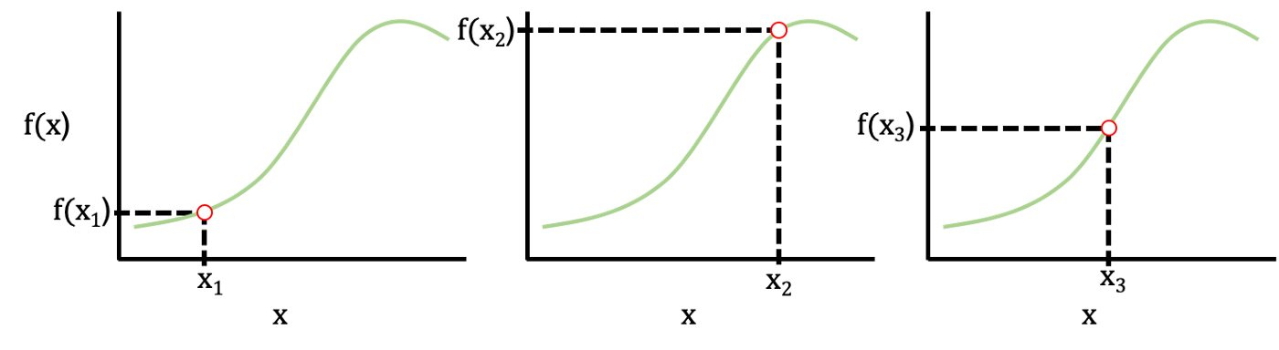
먼저, 우리는 몬테 카를로를 사용하여 적분의 기대값(expected value) 조사할 수 있습니다. 전통적으로, 함수 g(x)의 기대값은 먼저 확율밀도함수(probability density function)인 f(x)를 곱하고 원하는 영역의 적분하여 계산될 수 있습니다:

또는, 우리는 제한된 적분 영역 사이에서 균일한 분포로 반복해서 샘플링하므로써 기대값에 대한 몬테 카를로 근사를 사용할 수 있습니다.

언급한 것과 같이, 각각 유일한 n=1,2,3 등등에서, xi는 a와 b 사이로 제한된 균일한 분포에서 샘플링한 값입니다. 이런 접근법은 수렴하는 기대값(converged expected value)을 찾기 위해서 f(x) 함수를 샘플링하고 대수의 법칙(the law of large numbers)를 사용합니다.
As an aside, the multiplicative factor of 1/n is sometimes given as 1/(n-1) because there are truly n-1 degrees of freedom with n-samples, but when n is large enough the difference between 1/n and 1/(n-1) is negligible.
기대값에 대한 추정기의 형태가 주어지면, 적분의 추정치 까지 확장하는 것은 간단합니다. 기대값 공식은 아래 보는 것과 같이 적분의 제한 영역의 범위를 곱해줍니다.

적분의 추정치는 적분 면적/부피의 근사치를 찾기 위해서 적분의 제한 범위에 의해서 결정되어지는 사각형의 가로길이와 함께 기대값 추정기를 사용합니다.

우리는 비교적 간단한 예제에서 테스트할 수 있습니다, 적분을 구함:

분석적인 해결법(analytical solution)은 대략 ~13.340 입니다. 우리는 n=200인 샘플 크기로, 몬테 카를로 적분 기술을 적용하기 위해서 간단한 C++ 프로그램을 작성할 수 있습니다.
#include <iostream>
#include <cstdlib>
#include <cmath>

double myFunction(double x);
double monteCarloEstimate(double lowBound, double upBound, int iterations);

int main()
{

  double lowerBound, upperBound;
  int iterations;

  lowerBound = 1;
  upperBound = 5;
  iterations = 200;

  double estimate = monteCarloEstimate(lowerBound, upperBound,iterations);

  printf("Estimate for %.1f -> %.1f is %.2f, (%i iterations)\n",
      lowerBound, upperBound, estimate, iterations);

  return 0;
}

double myFunction(double x)
//Function to integrate
{
  return pow(x,4)*exp(-x);
}

double monteCarloEstimate(double lowBound, double upBound, int iterations)
//Function to execute Monte Carlo integration on predefined function
{

  double totalSum = 0;
  double randNum, functionVal;

  int iter = 0;

  while (iter<iterations-1)
  {

    //Select a random number within the limits of integration
    randNum = lowBound + (float(rand())/RAND_MAX) * (upBound-lowBound);

    //Sample the function's values
    functionVal = myFunction(randNum);

    //Add the f(x) value to the running sum
    totalSum += functionVal;

    iter++;
  }

  double estimate = (upBound-lowBound)*totalSum/iterations;

  return estimate;
}
이것과 가까운 결과를 출력할 것입니다:
Estimate for 1.0 -> 5.0 is 13.28, (200 iterations)특히 샘플의 크기가 n=200 정도임을 고려하면, 13.28의 추정치는 분석적인 해결법(analytical solution)인 ~13.34에서 크게 벗어나지 않습니다.
어떻게 몬테 카를로 적분법을 더 정확하게 수행하게 할 수 있나요? 이것에 대답하기 위해서, 우리는 몬테 카를로 적분 기술에 내포된 분산에 대해서 알아봐야 합니다.
Monte Carlo Integration: Variance
몬테 카를로 적분 형식의 분산은 특정 랜덤 변수의 주변의 분산을 계산하는 전통적인 처리 과정을 따릅니다.
간결하게 하기 위해, 나는 표준편차와 몬테 카를로 적분 형식과의 관계에 대한 유도는 생략하겠습니다. 만약 우리가 함수 g(x)의 적분을 구하는 이전 표기법을 계속 사용하면, g(x)의 적분의 기대값 주변의 분산은 다음과 같이 주어질 수 있습니다:
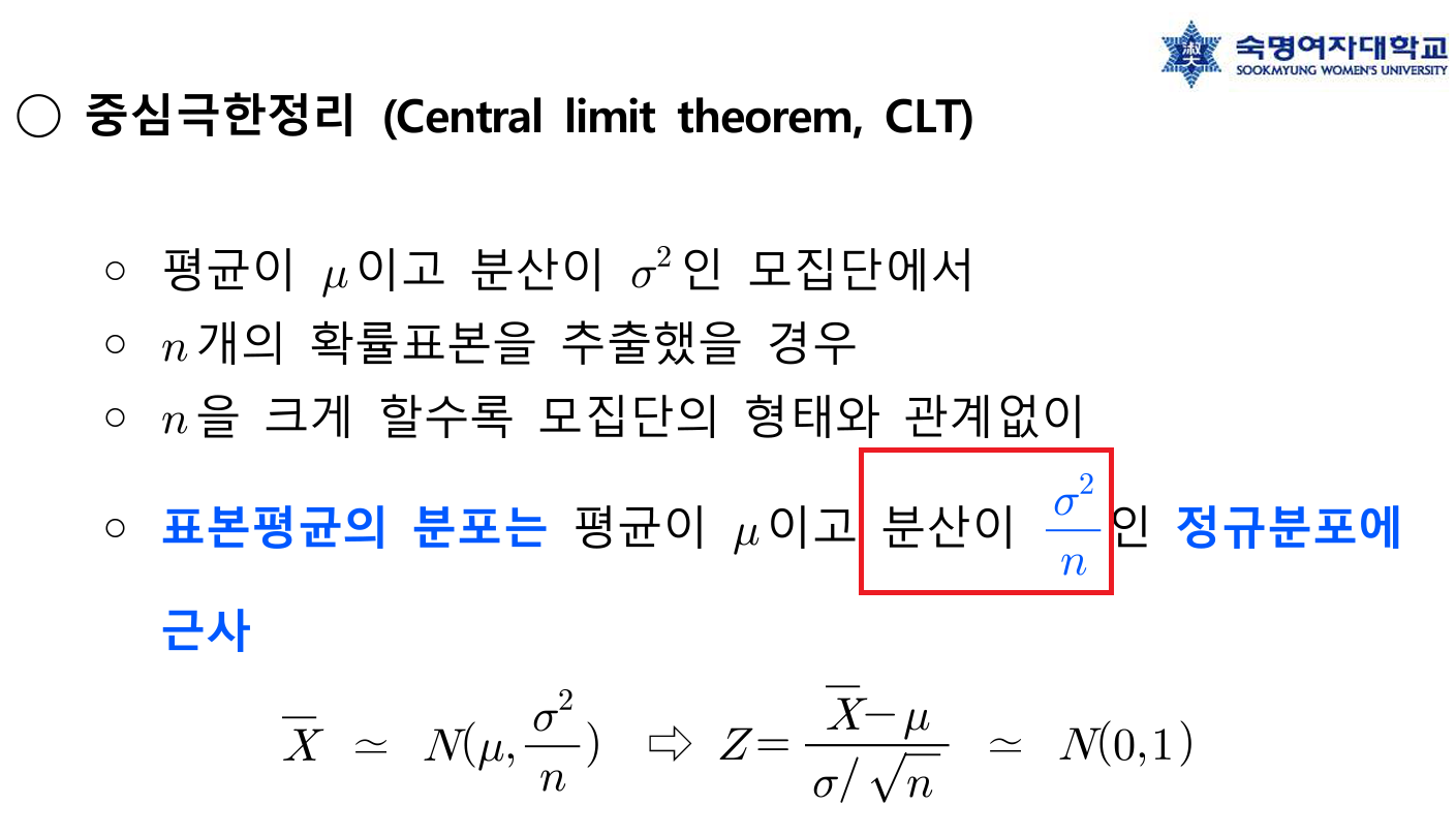
(역주1 : 개인적으로 이부분이 정확히 맞는지 모르겠습니다. 분산 = (제곱의 평균 - 평균의 제곱), 표준편차 = sqrt(분산) 라고 알고 있는데요. 아래 식에서 표준편차를 구하는 식의 근호 내에서 (n - 1)를 나눠주고 있습니다. 이 부분이 왜 그런지 정말 표준편차를 구하기 위한 식인지 궁금합니다.)
(역주2: "ROBUST MONTECARLO METHODS FOR LIGHTTRANSPORT SIMULATION - Eric Veach December 1997"의 39p "2.4.1 Convergence rates" 항목을 보면 표준편차가 1/sqrt(n) 에 비례하는 것을 확인 할 수 있습니다(역주 추가 그림1 참고). 또 다른 글에서는 중심극한정리(CLT)의 정의에 따르면 분산=표준편차제곱/n 이라 합니다(역주 추가 그림2 참고). 이 경우도 1/sqrt(n)입니다.)
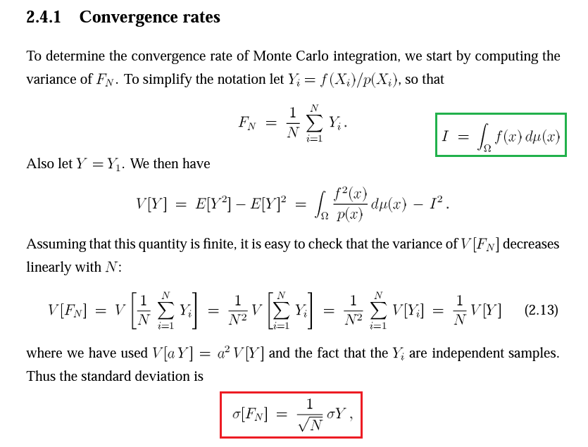

여기에 추가된 V 는 적분 제한 영역의 총 부피를 나타냅니다. 만약 제한된 a와 b 사이의 1 차원 적분을 한다면 다음과 같이 쓸 수 있습니다:

이런 형식을 사용하여, 우리는 적분 추정치와 함께 표준편차(표준편차^2 = 분산)나 분산을 쉽게 계산할 수 있습니다. 오차 방정식(the error equation)에서 예상되는 가장 명백한 결과 중 하나는 몬테 카를로 적분 추정기의 표준편차는 샘플의 수의 제곱근에 반비례 하는 것입니다.

그래서 우리는 추정치의 오차를 원한는 만큼 줄이기 위해서 어떻게 샘플의 크기를 증가시키냐에 대한 아이디어가 있습니다. 예를들면, 오차가 2배 감소하려면 샘플 수가 4배 증가해야 합니다!
그래서 에러 감소는 특히 다른 수치(numerical) 적분 형식과 비교하여 용인하기 어려운 과정입니다. 그러나, 다른 수치(numerical) 기법은 차원의 저주(the curse of dimensionality)에 의해 고통받습니다, 이것은 당신이 적분의 차원을 늘리면 함수의 오차는 기하급수적으로 나빠진다는 의미입니다. 대조적으로, 몬테 카를로 적분법은 적분 차원의 수와 관계없이 1/sqrt(n) 오차 배율을 유지합니다. 이런 점은 고차원 스케일링에 이상적입니다.
샘플 크기에 대해 추정된 오차의 비율을 나타내기 위해서, 우리는 점점 더 큰 샘플 크기의 표준편차를 계산하면서, 이전과 동일한 적분 예제를 사용할 수 있습니다. 우리는 n=8, 32, 128, 512, 2048(샘플 크기가 매번 4배씩 증가) 계산을 시도할 수 있습니다.
#include <iostream>
#include <cstdlib>
#include <cmath>

double myFunction(double x);
void monteCarloEstimateSTD(double lowBound, double upBound, int iterations, double mcStats[]);

int main()
{

  double lowerBound, upperBound;
  int iterations;

  lowerBound = 1;
  upperBound = 5;

  double mcStats[2]; //position 0 holds the estimate, position 1 holds the STD

  for(int i =1;i<6;i++)
  {

    iterations = 2*pow(4,i);

    monteCarloEstimateSTD(lowerBound, upperBound,iterations, mcStats);

    printf("Estimate for %.1f -> %.1f is %.3f, STD = %.4f, (%i iterations)\n",
      lowerBound, upperBound, mcStats[0], mcStats[1], iterations);

  }

  return 0;
}

double myFunction(double x)
//Function to integrate
{
  return pow(x,4)*exp(-x);
}

void monteCarloEstimateSTD(double lowBound, double upBound, int iterations, double statsArray[])
//Function to execute Monte Carlo integration on predefined function
{
  double totalSum = 0;
  double totalSumSquared = 0;

  int iter = 0;

  while (iter<iterations-1)
  {

    double randNum = lowBound + (float(rand())/RAND_MAX) * (upBound-lowBound);

    double functionVal = myFunction(randNum);

    totalSum += functionVal;
    totalSumSquared+= pow(functionVal,2);

    iter++;
  }

  double estimate = (upBound-lowBound)*totalSum/iterations;
  double expected = totalSum/iterations;

  double expectedSquare = totalSumSquared/iterations;

  double std = (upBound-lowBound)*pow( (expectedSquare-pow(expected,2))/(iterations-1) ,0.5);

  statsArray[0] = estimate;
  statsArray[1] = std;
}
이것과 같은 결과가 나올 것입니다:
Estimate for 1.0 -> 5.0 is 8.365, STD = 2.6452, (8 iterations)
Estimate for 1.0 -> 5.0 is 13.548, STD = 1.1617, (32 iterations)
Estimate for 1.0 -> 5.0 is 13.171, STD = 0.4994, (128 iterations)
Estimate for 1.0 -> 5.0 is 13.235, STD = 0.2542, (512 iterations)
Estimate for 1.0 -> 5.0 is 13.375, STD = 0.1243, (2048 iterations)
예상한대로 4배 증가된 샘플 크기는 추정기의 오차를 2배 감소시킵니다!
Variance Reduction
몬테 카를로 적분의 핵심 개념은 꽤 간단하며 알고리즘의 많은 수정은 정확한 추정치를 얻기위해서 통계적 오차와 샘플의 수를 줄이기 위한 것입니다 - 이런 방법들은 일반적으로 분산 감소 범주로 분류됩니다. 각각의 방법에 대해 자세히 들어가지는 않을 것입니다, 그러나 사용 가능한 다양한 유형의 최적화 절차에 대한 아이디어를 알고 있는 것은 어떤 것이 사용하기에 적합한지 파악하는데 도움이 될 수 있습니다.
Importance Sampling
이전에, 우리는 적분 제한 영역 사이에서 랜덤 균등 분포로 부터 샘플링 했습니다. 종종 함수는 적분값의 총합에서 무의미하게 작은 부분을 차지하는 '덜 중요한' 데이터 값의 영역을 가집니다. 만약 우리가 샘플 분포를 균등 분포에서 관심있는 함수와 다소 유사한 확률 밀도 함수로 조정할 수 있다면, 우리는 더 빠르게 통계적으로 신뢰할 수 있는 적분 추정치에 도달할 수 있고 샘플링 분산을 줄일 수 있습니다. 샘플링할 Companion function 을 선택하는 것은 간단하지 않습니다, 그리고 때때로 적분되고 있는 함수에 대한 사전지식이 요구됩니다.
적절한 Companion 확률 밀도 함수가 선택되어지면 (즉, p(x)), xi 값은 Companion distribution 으로 부터 샘플링 되어지고 적분 추정치는 새로운 샘플링 바이어스를 고려하는 곱셈 요소를 사용하여 계산되어집니다. 곱셉 요소는 때때로 Importance weight 라고 불려 집니다. Importance weight는 바이어스 된 샘플들이 여전히 추정치를 기대값으로 향하도록 보장합니다. Importance sampling 을 사용한 몬테 카를로 추정치의 일반적인 표현은 다음과 같습니다:

만약 우리가 적분 제한 영역 a와 b를 사용하는 균일 분포 샘플링으로 부터 변경한다고 가정하면, 우리는 균일 분포의 확률 밀도 함수를 PDF=1/(max-min)으로 사용하여 식을 더욱 간단히 할 수 있습니다.

예를들어, 아래에 주어진 함수와 그에 대응하는 그래프를 고려해봅시다. x=[0,6] 범위에서 정확한 기대값 또는 적분 추정치를 찾기를 원한다고 가정합니다.
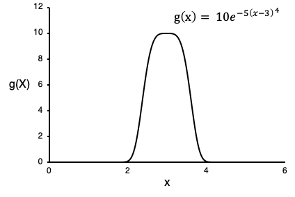
만약 무식한 방식으로 몬테 카를로 적분을 사용하면, x=[0,10]과 x=[4,6] 범위로 부터 얻은 샘플들은 피적분 함수가 높은 x=[2,4] 범위보다 더 많은 정보를 주지 않을 것입니다. 랜덤 변수를 샘플링 할 Companion function 는 g(x)의 모양과 일치해야 합니다. (x=[2,4] 에서 높은 샘플 확률을 가지고, 바깥 방향에서 줄어드는 관점에서) 그래서 예를들어 우리는 μ = 3 and σ = 1 을 사용하는 normal distribution 을 사용할 수 있습니다.

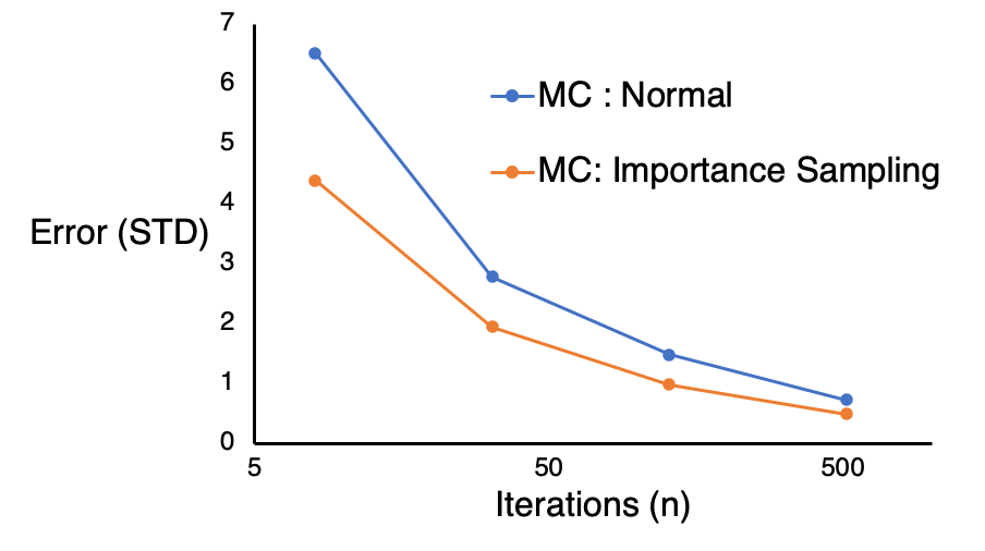
우리는 Importance sampling 을 사용하여 강화된 몬테 카를로 적분과 일반적인 몬테 카를로 적분의 성능을 비교하여 Companion function으로 부터의 샘플링이 어떻게 오차를 줄일 수 있는지 보여줄 수 있습니다:
#include <iostream>
#include <cstdlib>
#include <cmath>
#include <random>

double myFunction(double x);
double myPDF(double x);
void monteCarloEstimate(double lowBound, double upBound, int iterations, double mcStats[]);
void monteCarloEstimateImportance(double lowBound, double upBound, int iterations, double mcStats[]);

int main()
{
  double lowerBound, upperBound;
  int iterations;

  lowerBound = 1;
  upperBound = 5;

  double mcStats[2]; //position 0 holds the estimate, position 1 holds the STD
  double mcStatsImport[2]; //position 0 holds the estimate, position 1 holds the STD

  int num_trials = 4;

  //Print a table header
  printf("MC Normal Sampling\t\tMC Importance Sampling\t\tIterations\n");
  printf("Estimate\tSTD\t\tEstimate\tSTD\n");

  for(int i =1;i<=num_trials;i++)
  {
    iterations = 2*pow(4,i);

    monteCarloEstimate(lowerBound, upperBound,iterations, mcStats);
    monteCarloEstimateImportance(lowerBound, upperBound,iterations, mcStatsImport);

    printf("%.3f\t\t%.3f\t\t%.3f\t\t%.3f\t\t%i\n" ,
      mcStats[0], mcStats[1],mcStatsImport[0], mcStatsImport[1] ,iterations);
  }

  return 0;
}

double myFunction(double x)
//Function to integrate
{
  return 10*exp(-5*pow(x-3,4));
}

double myPDF(double x)
//Function to integrate
{
  return (1/pow(2*3.14159,0.5))*exp(-(0.5)*pow(x-3,2));
}

void monteCarloEstimate(double lowBound, double upBound, int iterations, double statsArray[])
//Function to execute Monte Carlo integration on predefined function
{
  double totalSum = 0;
  double totalSumSquared = 0;

  int iter = 0;
  while (iter<iterations-1)
  {
    double randNum = lowBound + (float(rand())/RAND_MAX) * (upBound-lowBound);
    double functionVal = myFunction(randNum);

    totalSum += functionVal;
    totalSumSquared+= pow(functionVal,2);

    iter++;
  }

  double estimate = (upBound-lowBound)*totalSum/iterations; //For normal solve
  double expected = totalSum/iterations;
  double expectedSquare = totalSumSquared/iterations;
  double std = (upBound-lowBound)*pow( (expectedSquare-pow(expected,2))/(iterations-1) ,0.5);

  statsArray[0] = estimate;
  statsArray[1] = std;
}

void monteCarloEstimateImportance(double lowBound, double upBound, int iterations, double statsArray[])
//Function to execute Monte Carlo integration on predefined function
{
  //Random number generator to generate samples from the companion distribution
  std::default_random_engine generator;
  std::normal_distribution<double> distribution(3,1.0);

  double totalSum = 0;
  double totalSumSquared = 0;

  int iter = 0;

  double randNum, functionVal;
  double weight;

  while (iter<iterations-1)
  {
    randNum = distribution(generator);
    weight = (1/(upBound-lowBound))/myPDF(randNum);
    functionVal = myFunction(randNum)*weight;

    totalSum += functionVal;
    totalSumSquared+= pow(functionVal,2);

    iter++;
  }

  double estimate = (upBound-lowBound)*totalSum/iterations;
  double expected = totalSum/iterations;
  double expectedSquare = totalSumSquared/iterations;
  double std = (upBound-lowBound)*pow( (expectedSquare-pow(expected,2))/(iterations-1) ,0.5);

  statsArray[0] = estimate;
  statsArray[1] = std;
}
우리는 그래프를 사용하여 오차 vs 반복수를 보여줄 수 있으며 importance sampling 을 사용하여 모든 케이스에서 샘플링의 표준 편차를 줄일 수 있는 것을 볼 수 있습니다.
Importance sampling은 특히 피적분 함수의 형태에 대해서 아는 것이 적을 때는 쉽지 않습니다. 만약 주의하지 않는다면, 오차가 폭발하거나 심지어 무한대로 갈 수 있습니다.
Stratified Sampling
Stratified sampling은 적분 볼륨이 각각 분리되어 평가되는 서브 도메인으로 나뉘어지는 분산 감소에 대한 또 다른 접근입니다. 각각의 서브도메인의 추정치는 그들의 서브도메인 적분 볼륨에 따라 가중치를 사용하여 조합됩니다. Stratified sampling 은 함수의 모양에 대한 사전지식 없이 항상 샘플 분산을 감소시키는 장점이 있습니다. 최적화된 stratified sampling 절차는 특정 peaks나 값을 그룹화하여 유사한 값을 가진 영역으로 함수를 재귀적으로 나누는 것입니다. 마찬가지로, 함수 구조의 사전 지식 없이 적분 볼륨을 균일한 큰 작업으로 파싱하는 단순한(naive) 접근방식 입니다.
함수 g(x) 적분의 Stratified sampling 추정치는 다음과 같습니다:

여기서, 원본 샘플 볼륨은 k 서브 도메인으로 나뉘어집니다, 각각의 j 번째 서브 모듈은 V_j 볼륨과 n_j 샘플을 얻습니다. 표준편차의 표현은 다음과 같이 수정됩니다:

σ_j 는 각각의 j 번째 서브 도메인 범위 내에 있는 샘플들의 표준편차입니다.
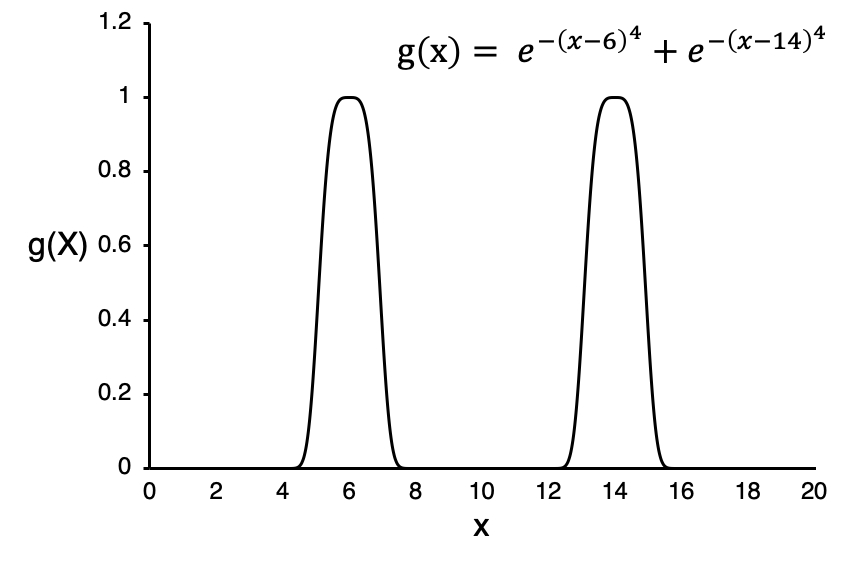
Stratified sampling 의 간단한 예제는 아래의 그림에 적용할 수 있습니다, 여기서 적분 범위를 5개의 동일 크기의 영역으로 나눌 것입니다 (즉, x=[0,4], x=[4,8], x=[8,12], x=[12,16], x=[16,20]).
아래의 코드는 일반적인 몬테 카를로 적분과 Stratified Sampling 을 비교합니다.
#include <iostream>
#include <cstdlib>
#include <cmath>

double myFunction(double x);
void monteCarloEstimateSTD(double lowBound, double upBound, int iterations, double mcStats[]);
void monteCarloEstimateStrat(double lowBound, double upBound, int iterations, double mcStats[], int subdomains);

int main()
{
  double lowerBound, upperBound;
  int iterations;

  lowerBound = 0;
  upperBound = 20;

  double mcStats[2]; //position 0 holds the estimate, position 1 holds the STD

  printf("Normal Monte Carlo Integration\n");
  for(int i =1;i<6;i++)
  {
    iterations = 128*pow(4,i);
    monteCarloEstimateSTD(lowerBound, upperBound,iterations, mcStats);

    printf("Estimate for %.1f -> %.1f is %.3f, STD = %.4f, (%i iterations)\n",
      lowerBound, upperBound, mcStats[0], mcStats[1], iterations);
  }

  printf("Stratified Sampling Monte Carlo Integration\n");
  for(int i =1;i<6;i++)
  {
    iterations = 128*pow(4,i);
    monteCarloEstimateStrat(lowerBound, upperBound,iterations, mcStats,4);

    printf("Estimate for %.1f -> %.1f is %.3f, STD = %.4f, (%i iterations)\n",
      lowerBound, upperBound, mcStats[0], mcStats[1], iterations);
  }
  return 0;
}

double myFunction(double x)
//Function to integrate
{
  return exp(-1*pow(x-6,4)) +  + exp(-1*pow(x-14,4));
}

void monteCarloEstimateSTD(double lowBound, double upBound, int iterations, double statsArray[])
//Function to execute Monte Carlo integration on predefined function, calculates STD
{
  double totalSum = 0;
  double totalSumSquared = 0;
  int iter = 0;

  while (iter<iterations-1)
  {
    double randNum = lowBound + (float(rand())/RAND_MAX) * (upBound-lowBound);
    double functionVal = myFunction(randNum);

    totalSum += functionVal;
    totalSumSquared+= pow(functionVal,2);

    iter++;
  }

  double estimate = (upBound-lowBound)*totalSum/iterations; //For normal solve
  double expected = totalSum/iterations;
  double expectedSquare = totalSumSquared/iterations;
  double std = (upBound-lowBound)*pow( (expectedSquare-pow(expected,2))/(iterations-1) ,0.5);

  statsArray[0] = estimate;
  statsArray[1] = std;
}

void monteCarloEstimateStrat(double lowBound, double upBound, int iterations, double statsArray[], int subdomains)
//Function to execute Monte Carlo integration on predefined function, uses stratified sampling of equally sized subdomains
{
  double totalSum[subdomains];
  double totalSumSquared[subdomains];
  int iter;

  //Divide the local iterations amoung the subdomains
  iterations = int( float(iterations)/subdomains);

  for(int i = 0;i<subdomains;i++)
  {
    totalSum[i]=0;
    totalSumSquared[i]=0;
  }

  //Amount of change the range by each time
  double increment = (upBound-lowBound)/float(subdomains);

  for(int seg = 0;seg<subdomains;seg++)
  {
    iter = 0;
    double randNum;
    double functionVal;
    double startRange = lowBound+seg*increment;

    while (iter<iterations-1)
    {
      randNum = startRange + (float(rand())/RAND_MAX) * increment;
      functionVal = myFunction(randNum);

      totalSum[seg] += functionVal;
      totalSumSquared[seg] += pow(functionVal,2);

      iter++;
    }
  }

  double estimates[subdomains];
  double expecteds[subdomains];
  double expectedSquares[subdomains];
  double STDs[subdomains];

  for(int i = 0;i<subdomains;i++)
  {
    estimates[i] = increment*totalSum[i]/iterations; //For normal solve
    expecteds[i] = totalSum[i]/iterations;
    expectedSquares[i] = totalSumSquared[i]/iterations;

    STDs[i] = increment*pow( (expectedSquares[i]-pow(expecteds[i],2))/(iterations-1) ,0.5);
  }

  double estimate=0;
  double std=0;

  for(int i = 0;i<subdomains;i++)
  {
    estimate += estimates[i];

    // (역주3. pow(STDs[i], 2)는 STDs[i]가 되어야 하는게 아닌가 함. 위의 공식에는 제곱을 하지 않음.)
    std += pow(increment,2)*pow( STDs[i] ,2)/iterations;
  }

  statsArray[0] = estimate;
  statsArray[1] = pow(std,0.5);
}
Normal Monte Carlo Integration
Estimate for 0.0 -> 20.0 is 2.697, STD = 1.6518, (16 iterations)
Estimate for 0.0 -> 20.0 is 4.057, STD = 0.8851, (64 iterations)
Estimate for 0.0 -> 20.0 is 3.715, STD = 0.4479, (256 iterations)
Estimate for 0.0 -> 20.0 is 3.591, STD = 0.2133, (1024 iterations)
Estimate for 0.0 -> 20.0 is 3.388, STD = 0.1053, (4096 iterations)
Estimate for 0.0 -> 20.0 is 3.579, STD = 0.0538, (16384 iterations)

Stratified Sampling Monte Carlo Integration
Estimate for 0.0 -> 20.0 is 1.125, STD = 1.8661, (16 iterations)
Estimate for 0.0 -> 20.0 is 2.113, STD = 0.7077, (64 iterations)
Estimate for 0.0 -> 20.0 is 3.860, STD = 0.1922, (256 iterations)
Estimate for 0.0 -> 20.0 is 3.439, STD = 0.0464, (1024 iterations)
Estimate for 0.0 -> 20.0 is 3.689, STD = 0.0116, (4096 iterations)
Estimate for 0.0 -> 20.0 is 3.612, STD = 0.0029, (16384 iterations)
두 접근법의 오차를 그림으로 나타낸다면, stratified sampling 이 이점을 있다는 것이 명확할 것입니다.

읽어주셔서 감사합니다 - 어떠한 제안이나 수정도 환영합니다! mediumCameron@gmail.com 으로 연락해주세요.
References
- Lisovskaja, Vera. Mathematical Statistics, Chalmers — TMS150, Stochastic Data Processing and Simulation, www.math.chalmers.se/Stat/Grundutb/CTH/tms150/1112/.
- Jarosz, Wojciech. “Efficient Monte Carlo Methods for Light Transport in Scattering Media.” UC San Diego, 2008, cs.dartmouth.edu/~wjarosz/publications/dissertation/.
- “Monte Carlo Method.” Wikipedia, Wikipedia, https://en.wikipedia.org/wiki/Monte_Carlo_method
반응형
'Graphics > 참고자료' 카테고리의 다른 글
| [번역] Multiple Importance Sampling in 1D (0) | 2022.04.11 |
|---|---|
| [번역] Monte Carlo Integration Explanation in 1D (0) | 2022.04.09 |
| [번역] Your Guide to Texture Compression in Unreal Engine (0) | 2021.10.29 |
| [번역] Visibility Buffer Rendering with Material Graphs – Filmic Worlds (2) | 2021.10.15 |
| [번역] Temporal Anti-Aliasing(TAA) Tutorial (0) | 2021.06.24 |
'Graphics/참고자료' Related Articles
more


